
In most countries, fixed feed-in compensation for renewable energies is replaced by alternative models. Greater market integration is the primary driver. Right now, the Power Purchase Agreement (PPA) is an alternative compensation form that receives much attention. This article explains the different types of PPAs and shows how they can be considered in financial planning.
Power Purchase Agreements describe a mostly long-term agreement between an electricity producer and consumer. This agreement defines all commercial conditions between both parties and varies in form, delivery structure, pricing, or maturity. Compared to fixed feed-in compensation, financial models face new requirements.
Difference between physical and virtual PPAs
A distinction is made between physical and virtual PPAs. The physical PPA creates an obligation to deliver the agreed electricity physically. The virtual or financial PPA describes a ‘contract of difference’. In this case, there is no obligation to deliver electricity physically. In both cases, a price is agreed upon conclusion of the contract. Under the physical PPA, electricity is delivered at this price. Under the virtual PPA, a payoff worth the difference between the market price and the agreed price is paid. The electricity producer must pay compensation if the market price is higher than the one agreed. The consumer must pay off if the agreed price is higher than the market price.
PPA delivery structures
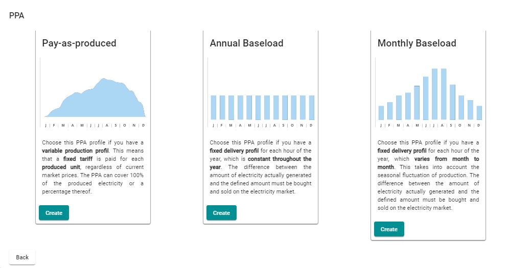
PPAs can have different delivery structures concerning the delivery obligation. Financial modelling distinguishes between two categories: Pay-as-Produced PPA and Fixed-Volume PPA.
Pay-As-Produced PPA
In the case of Pay-as-Produced PPA, the consumer buys an agreed share (ρ) of the electricity produced within this period (QActual) at a fixed price (PPPA). The remaining share of the produced electricity (1 – ρ) is sold at going price (PMarket) on the market. This mechanism can be easily depicted in a financial model. The expected income (R) is calculated as follows:
(1) R = ρ x PPPA + (1 – ρ) x PMarket
Once the electricity share (ρ) agreed in the PPA is supplemented by a cap, floor, or collar component, the calculation becomes somewhat more complicated. In this case, the consumer buys the agreed electricity share. However, the total amount is restricted by a cap, floor, or collar. For example, suppose a floor as a minimum amount is agreed (QPPA). In that case, the missing quantity must be procured for the current market price in case of QActual < QMin. The expected income, for this case, is calculated as follows:
(2) RActual < Min = QMin x PPPA – (QMin – QActual) x PMarket
Fixed-Volume PPA
For a Fixed-Volume PPA (sometimes also referred to as profile-based PPA), both parties agree on a fixed electricity amount (QPPA), which must be delivered by the producer. This involves for example ‘annual baseload’, ‘monthly baseload’, or ‘pre-defined solar’ contracts. The producer bears the so-called profile risk. Should a plant produce less than needed for the PPA, the rest must be purchased from the market at its going price (PMarket). The financial model evaluates for each period if the produced amount (QActual) is greater, lesser, or matches the delivery obligation. The expected income (R) is then calculated as follows:
(3) RActual < PPA = QPPA x PPPA – (QPPA – QActual) x PMarket
(4) RActual > PPA = QPPA x PPPA + (QActual – QPPA) x PMarket
(5) RActual = PPA = QPPA x PPPA
Profile overlap share
One challenge of the fixed PPAs with financial modelling is that they tend to come with a monthly resolution. The delivery obligation following the PPA often relates to much shorter periods, for example, hourly. Thus, monthly delivery obligations can be generally fulfilled. However, there might be hours within the month where delivery is not possible. The financial model must consider if the average market selling price (PSell) deviates from the average market purchase price (PBuy). There is no point to create a financial model on an hourly basis, which is why we model this effect using the profile overlap share.
Example: In January, the annual delivery obligation for each hour is 1,000MWh. For 744 hours, a total of 744,000MWh (QPPA) can be calculated for January. Suppose the plant produces 1,500MWh in the first 372 hours, and 500MWh for the remaining 372 hours. In total, the plant produces 744,000MWh (QActual) in January. Following this example, the first 372 hours with 1,000MWh are sold as part of the PPA, and the remaining 500MWh on the market. However, in the second half of January, each hour with 500MWh must be purchased on the market to fulfil the delivery obligation. Thus, the PPA delivery obligation is covered to 75% (profile overlap share) only (1 – (372 * 500MWh / 744,000MWh) = 75%).
With the help of the profile overlap share, the income is calculated as follows:
(6) R = QPPA x PPPA – (1 – μ) x PBuy + (1 – μ) x PSell
It can be ignored if the average electricity sales price (PSell) corresponds precisely to the average purchase price (PSell = PBuy). As a result, formula (6) is simplified to (7) and corresponds to (5) precisely:
(7) R = QPPA x PPPA
PPA price mechanisms
Delivery obligations and various prices must be considered when modelling PPAs. Three prices are crucial for this: PPA price, sales and purchase market price. The PPA price is the one agreed between both parties for the amount to be delivered. It can be fixed or variable. In many cases, a variable price comes with a cap, floor or collar (see above).
Cannibalisation effect & capture prices for renewable energy
Based on their substantial increase, renewable energies make up an increasingly larger share of the overall generation capacity. Thus, renewable energies have an increasing influence on wholesale electricity prices. As a result, prices fall in markets where renewable energies make up a significant share if they produce much electricity. It is referred to as the cannibalisation effect, often indicated as cannibalisation factor. The financial model must account for this connection. For this, the capture prices (PC) are used. The capture price is the achievable average market price for the specific technology. It can be calculated using the cannibalisation factor (δ) and average baseload-price (PMarket):
(8) PC = δ x PMarkt
As a result, the capture price is used in the financial model as sales price (PSell) for the electricity to be sold on the market.
Example: The average baseload-price is EUR 40MWh. The cannibalisation factor for wind energy projects is 90%. The capture price is EUR 36/MWh (EUR 40MWh * 90%).
Summary
PPAs offer the plant operator an additional option to protect against market price risks. Based on the diverse contract arrangements, financial modelling faces additional challenges. The aim is to transform the shorter electricity market cycles into the long-term financial model. Delivery structure and pricing concerning PPA design are central to this. Future capture prices can have significant long-term effects on project profitability as well, which is why it must be included in the modelling.
Do you need help with the financial modelling of PPAs? We are here to help! Arrange a personal consultation with one of our experts today!